Satellite sea surface temperature and chlorophyll-a in the Northeast Pacific

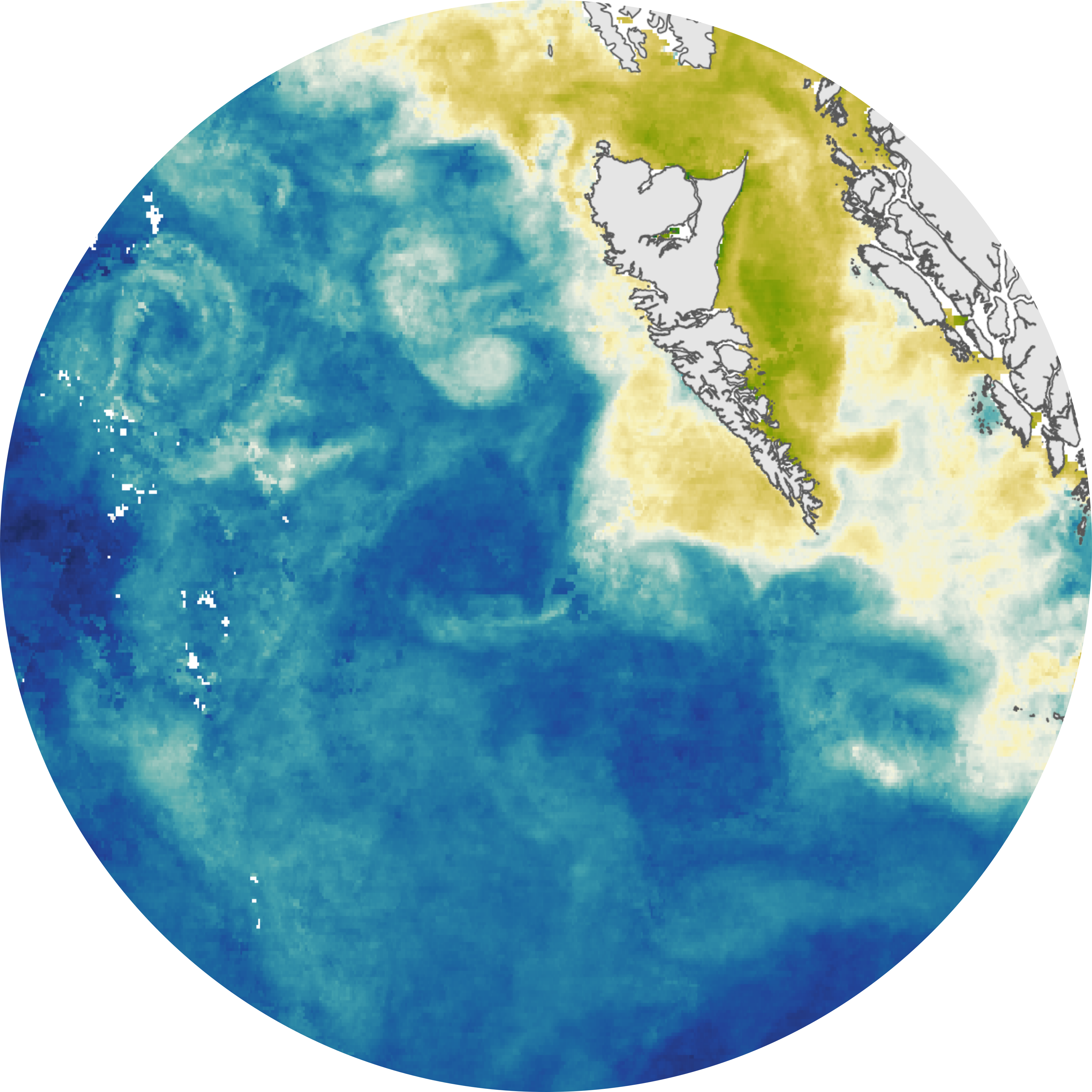
The ocean can be monitored at wide spatial scales using sensors on satellites. Satellites revisit much of the global ocean at least once per day, and data records now span decades. This allows scientists to look at long-term changes in the ocean. Satellite data can also be acquired from locations that cannot often be visited by ships, or autonomous sensors like gliders (see Ross et al. 2025) or Argo floats.

An image of mixed phytoplankton. Image from Wikimedia Commons, license CC BY SA 2.0.

Satellite surface chlorophyll-a concentration is used to approximate the biomass of phytoplankton in the upper ocean.

Sea surface temperature (SST) is one variable that satellites measure, during both daytime and night-time. Night-time SST is often used for analysis over the longer term, as it does not have diurnal heating, or the daily effect of the sun warming the surface of the water. SST records are useful for monitoring ocean heat events like Marine Heatwaves (MHWs).

Note

You can find more information and recent data on Marine Heatwaves in the Pacific region at this link.

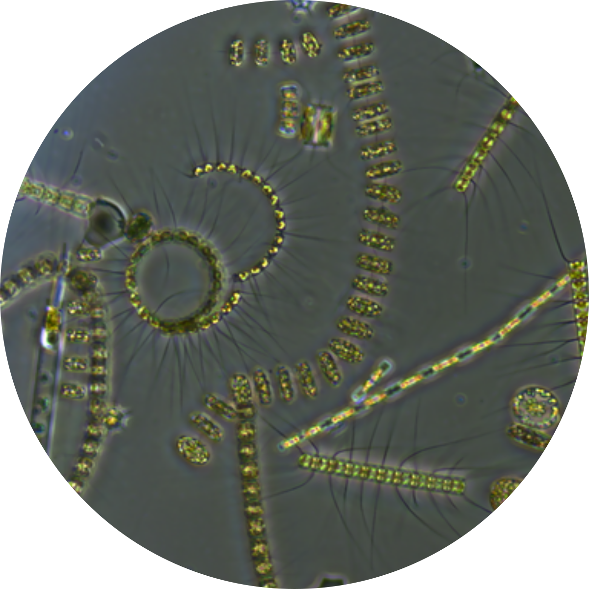
Chlorophyll-a (Chl-a), another parameter that satellites measure, is the dominant pigment in phytoplankton. Phytoplankton, tiny organisms that are found throughout the ocean, provide food to thousands of marine species, and make a large proportion of the world’s oxygen through photosynthesis.

How to use this site

This site updates monthly with maps and figures of SST and Chl-a, for monitoring their anomalies and values over the course of the year along the BC coast. Monitoring regions include Marine Protected and Conserved Areas, which supports reporting for Canada’s Marine Conservation Targets (MCT):

• GH: East (GHE), Offshore (GHO), South (GHS), West (GHW) Gwaii Haanas National Park Reserve, National Marine Conservation Area Reserve, and Haida Heritage Site

• SI: Scott Islands marine National Wildlife Area

• SK-B: SGaan Kinghlas-Bowie Seamount MPA

• SR: Central (SRC), North (SRN), South (SRS) Hecate Strait/Queen Charlotte Sound Glass Sponge Reefs MPA

• TḥT: Tang.ɢwan – ḥač^xwiqak – Tsig̱is MPA

For more information on MCT and MPAs, a comprehensive summary is also available in the latest version of The Current (pdf here📰).

Chl-a and SST in 2025

Region boundaries shown on weekly Chl-a from 2025. Since the region is very cloudy, satellite images are averaged together to improve spatial coverage of the data.

2025

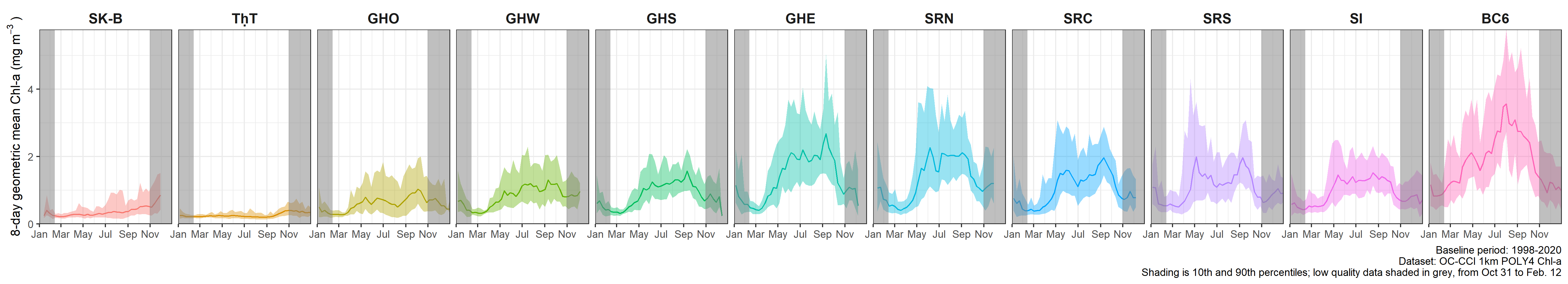
Chlorophyll-a

Sea surface temperature

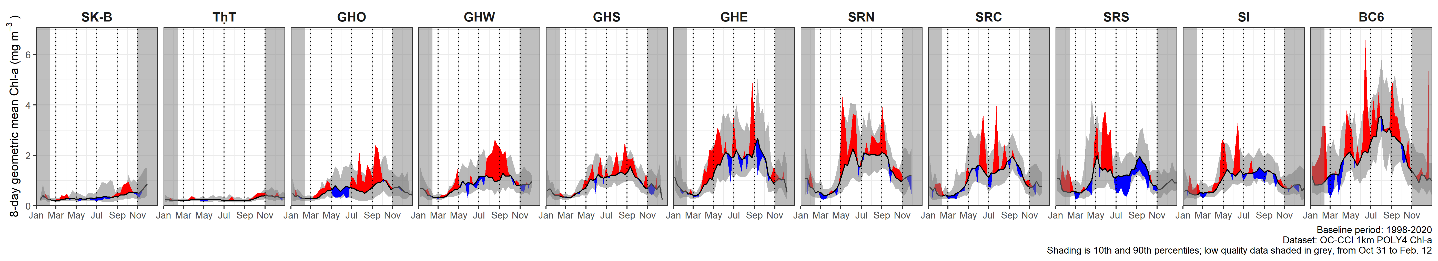
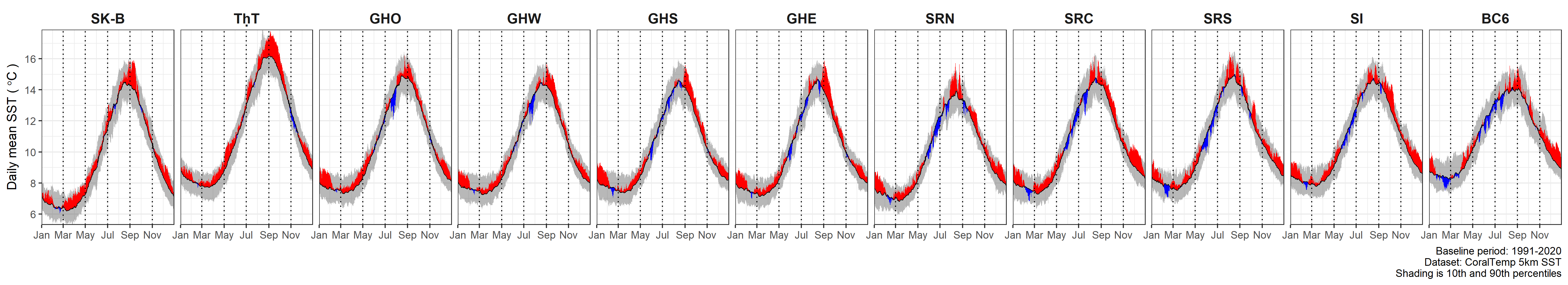The long-term averages are shown as a black line, with 10th and 90th percentiles as the grey shading. 2025 values are compared to this long-term average, with values higher shown in red and lower shown in blue.

For Chl-a, since the satellite record starts in 1997, the years 1998-2020 are used for the long-term average. 1991-2020, the Canadian Climate Normals period, is used for SST.

Long-term average

Chlorophyll-a

Sea surface temperature

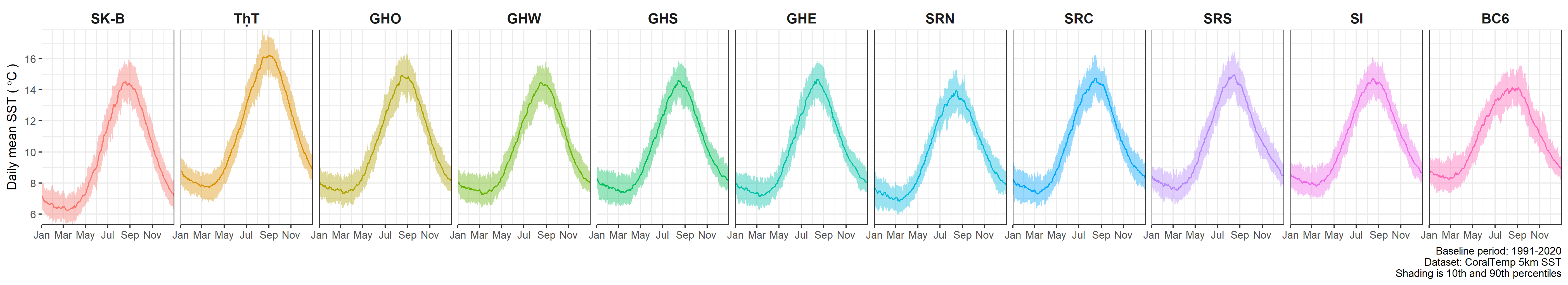The long-term averages are shown, with 10th and 90th percentiles as the coloured shading.

For Chl-a, since the satellite record starts in 1997, the years 1998-2020 are used for the long-term average. 1991-2020, the Canadian Climate Normals period, is used for SST.

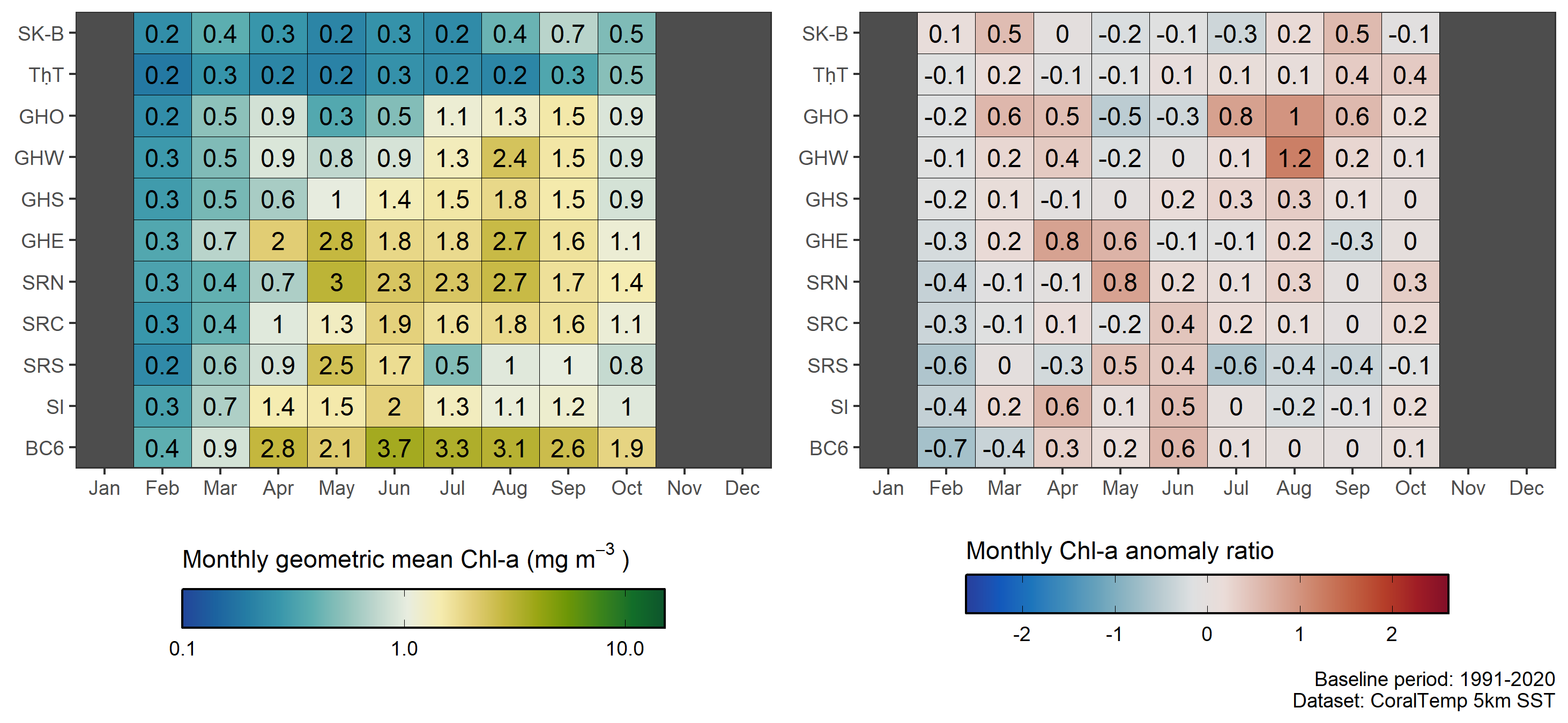
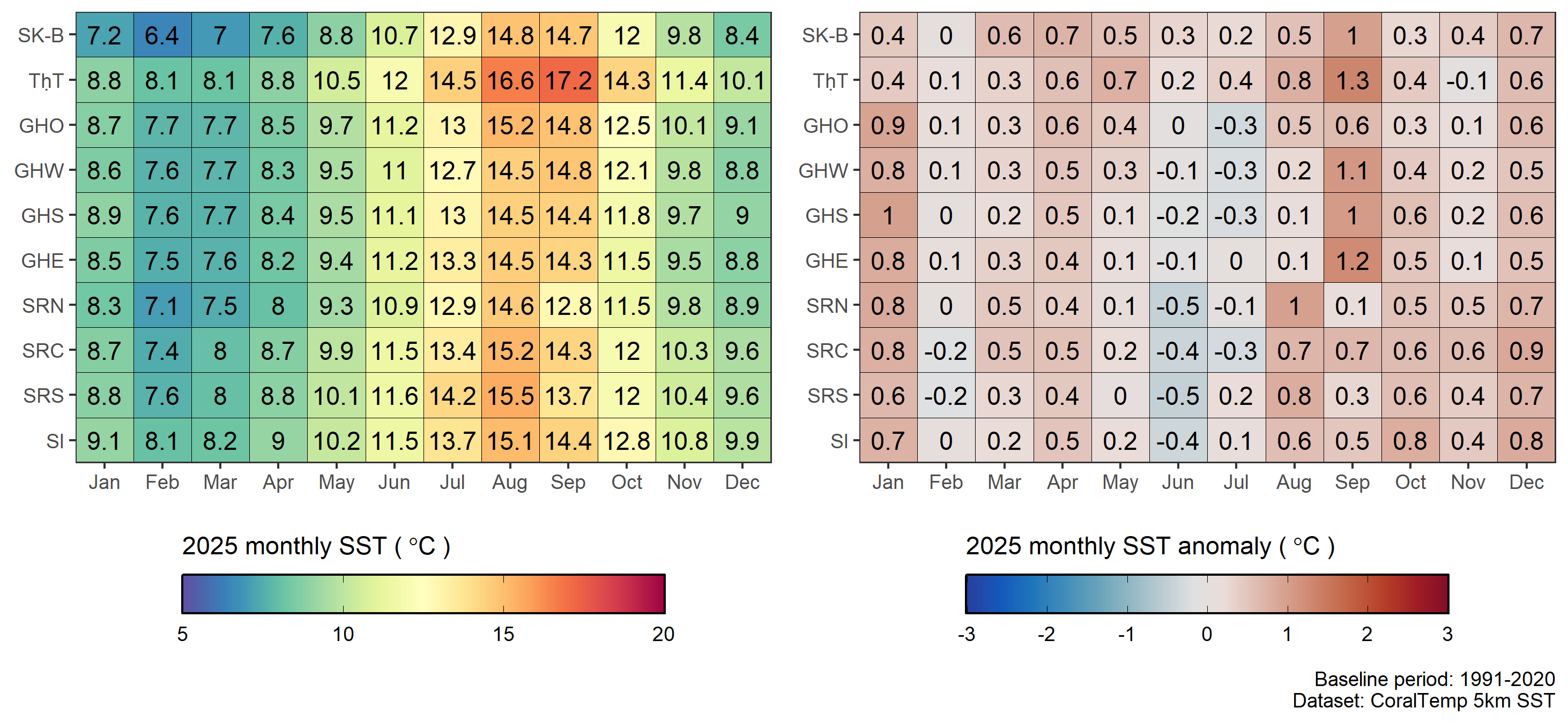
Monthly summaries and anomalies

Below, are monthly averages of chlorophyll-a (Chl-a) and sea surface temperature (SST) by region (left), and their anomalies compared to baseline monthly conditions (right).

In 2025, many regions had higher than normal Chl-a. For GHE and SRN, this was during April and May, while in GHO and GHW, during July and August. SST was generally warmer than normal, except in February in more southern regions, in June, and in many regions during July.

Note on Chl-a anomalies

🔎 For Chl-a, which has a log-normal distribution in the ocean (Campbell 1995), the anomaly was calculated as the anomaly ratio (as in Wang et al. 2021).

• Here, a value of 0.1, for example, indicates Chl-a was 10% higher than normal, and -0.2 is 20% lower than normal.

• Rather than calculating the anomaly as the baseline subtracted from the Chl-a value, which under-estimates year to year differences in Chl-a for lower productivity months or regions, the difference is also divided by the baseline. This method emphasizes the proportionate differences, which is more suitable for Chl-a, since biomass is so dynamic and increases rapidly during blooms.

📡Late fall and winter data, from November until early February, are also removed from the Chl-a dataset (indicated in grey shading in the figures). The low sun angle during this time of year causes more data loss and inaccuracy in optical satellite Chl-a measurements.

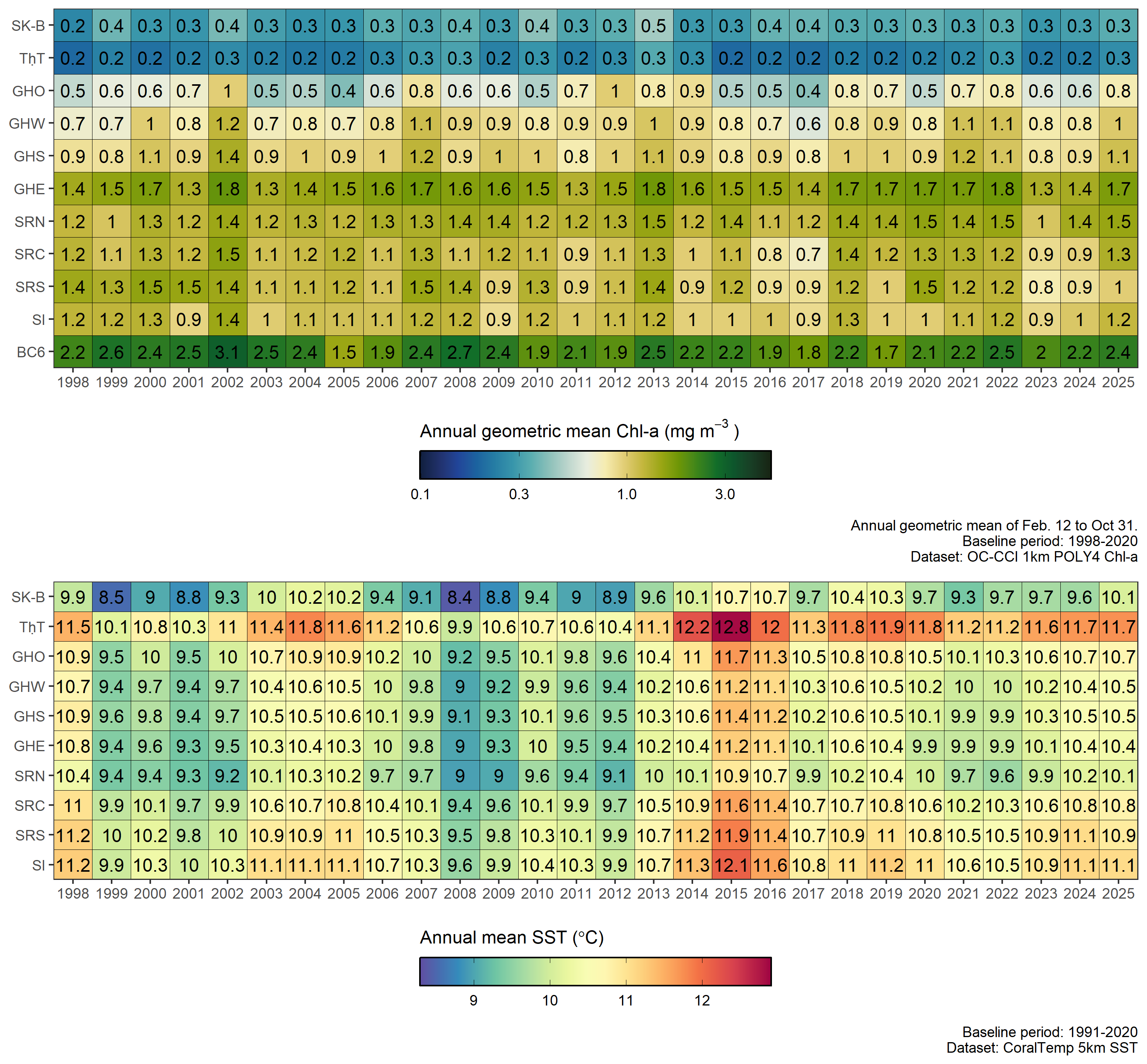
Annual summaries and anomalies

When averaged annually, overall changes in Chl-a and SST from year-to-year become more evident. Regional Chl-a shows the phytoplankton biomass differences between the offshore regions (SK-B and TḥT), which have low biomass, compared to the remaining regions mainly located on the shelf. GHE and BC6 have the highest phytoplankton biomass overall.

SST shows the impact of “the Blob” Marine Heatwave event that began in 2014 and ended in 2016. This event had widespread negative effects on Northeast Pacific ecosystems, from phytoplankton to whales and sea lions. Over half of Alaska’s common murres died during this event (Renner et al. 2024), there were widespread hamful algae blooms (Zhu et al. 2017), and record numbers of sea lions were starved and stranded.

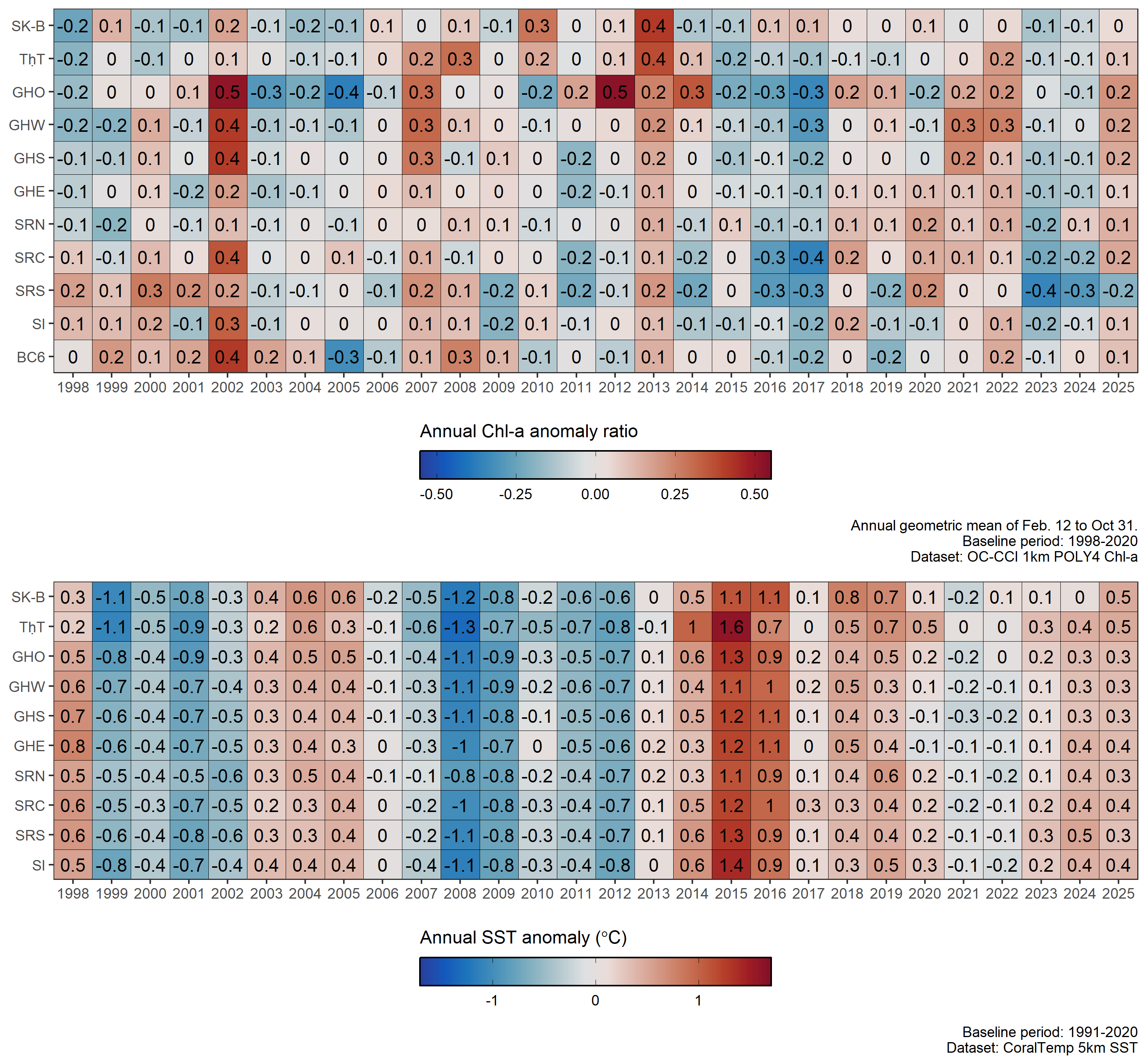
Chl-a and SST anomalies, where a given value is compared to its long-term average, differ more greatly from one another. SSTs, since late 2013, have largely been comparable to, or higher than, their long-term average. SST is typically closely related to El Niño–Southern Oscillation (ENSO), a natural climate phenomenon where winds and SSTs cyclically vary in the tropical Pacific. In the Northeast Pacific, El Niño years tend to be warmer than normal, while La Niña years tend to be cooler and wetter. However, in recent years, the cooling effects of La Niña have been less significant.

Further reading

We provide summaries of SST and Chl-a at the annual State of the Pacific Ocean (SOPO) meeting and published as a series of technical reports. The most recent SOPO meeting was held in March, 2026, with a technical report to be published in the coming months. For broader reading about the State of the Canada’s Oceans, check out the Canada’s Oceans Now report. 🌊🐟

Recent SOPO publications:

• Boldt, J.L., Joyce, E., Tucker, S., Gauthier, S., and Jackson, J. (Eds.). 2025. State of the physical, biological and selected fishery resources of Pacific Canadian marine ecosystems in 2024. Can. Tech. Rep. Fish. Aquat. Sci. 3687: viii + 337 p. https://doi.org/10.60825/hxdg-q818

• Boldt, J.L., Joyce, E., Tucker, S., Gauthier, S., and Dosser, H. (Eds.). 2024. State of the physical, biological and selected fishery resources of Pacific Canadian marine ecosystems in 2023. Can. Tech. Rep. Fish. Aquat. Sci. 3598: viii + 315 p.

References

Campbell, Janet. 1995. “The Lognormal Distribution as a Model for Bio-Optical Variability in the Sea.” Journal of Geophysical Research: Oceans 100 (C7): 13237–54. https://doi.org/10.1029/95JC00458.

Renner, Heather, John Piatt, Martin Renner, Brie Drummond, Jared Laufenberg, and Julia Parrish. 2024. “Catastrophic and persistent loss of common murres after a marine heatwave.” Science 386 (6727): 1272–76. https://doi.org/10.1126/science.adq4330.

Ross, Tetjana, Hayley Dosser, Jody Klymak, Wiley Evans, Alex Hare, Jennifer Jackson, and Stephanie Waterman. 2025. “Ocean Gliders for Planning and Monitoring Remote Canadian Pacific Marine Protected Areas.” Oceanography. https://doi.org/10.5670/oceanog.2025e104.

Wang, Menghua, Lide Jiang, Karlis Mikelsons, and Xiaoming Liu. 2021. “Satellite-Derived Global Chlorophyll-a Anomaly Products.” International Journal of Applied Earth Observation and Geoinformation 97 (May): 102288. https://doi.org/10.1016/j.jag.2020.102288.

Zhu, Zhi, Pingping Qu, Feixue Fu, Nancy Tennenbaum, Avery O. Tatters, and David A. Hutchins. 2017. “Understanding the Blob Bloom: Warming Increases Toxicity and Abundance of the Harmful Bloom Diatom Pseudo-Nitzschia in California Coastal Waters.” Harmful Algae 67 (July): 36–43. https://doi.org/10.1016/j.hal.2017.06.004.